XGBoost is an efficient implementation of gradient boosting for classification and regression problems.
It is both fast and efficient, performing well, if not the best, on a wide range of predictive modeling tasks and is a favorite among data science competition winners, such as those on Kaggle.
XGBoost can also be used for time series forecasting, although it requires that the time series dataset be transformed into a supervised learning problem first. It also requires the use of a specialized technique for evaluating the model called walk-forward validation, as evaluating the model using k-fold cross validation would result in optimistically biased results.
In this tutorial, you will discover how to develop an XGBoost model for time series forecasting.
After completing this tutorial, you will know:
- XGBoost is an implementation of the gradient boosting ensemble algorithm for classification and regression.
- Time series datasets can be transformed into supervised learning using a sliding-window representation.
- How to fit, evaluate, and make predictions with an XGBoost model for time series forecasting.
Kick-start your project with my new book XGBoost With Python, including step-by-step tutorials and the Python source code files for all examples.
Let’s get started.
- Update Aug/2020: Fixed bug in the calculation of MAE, updated model config to make better predictions (thanks Kaustav!)

How to Use XGBoost for Time Series Forecasting
Photo by gothopotam, some rights reserved.
Tutorial Overview
This tutorial is divided into three parts; they are:
- XGBoost Ensemble
- Time Series Data Preparation
- XGBoost for Time Series Forecasting
XGBoost Ensemble
XGBoost is short for Extreme Gradient Boosting and is an efficient implementation of the stochastic gradient boosting machine learning algorithm.
The stochastic gradient boosting algorithm, also called gradient boosting machines or tree boosting, is a powerful machine learning technique that performs well or even best on a wide range of challenging machine learning problems.
Tree boosting has been shown to give state-of-the-art results on many standard classification benchmarks.
— XGBoost: A Scalable Tree Boosting System, 2016.
It is an ensemble of decision trees algorithm where new trees fix errors of those trees that are already part of the model. Trees are added until no further improvements can be made to the model.
XGBoost provides a highly efficient implementation of the stochastic gradient boosting algorithm and access to a suite of model hyperparameters designed to provide control over the model training process.
The most important factor behind the success of XGBoost is its scalability in all scenarios. The system runs more than ten times faster than existing popular solutions on a single machine and scales to billions of examples in distributed or memory-limited settings.
— XGBoost: A Scalable Tree Boosting System, 2016.
XGBoost is designed for classification and regression on tabular datasets, although it can be used for time series forecasting.
For more on the gradient boosting and XGBoost implementation, see the tutorial:
First, the XGBoost library must be installed.
You can install it using pip, as follows:
sudo pip install xgboost
Once installed, you can confirm that it was installed successfully and that you are using a modern version by running the following code:
# xgboost
import xgboost
print("xgboost", xgboost.__version__)
Running the code, you should see the following version number or higher.
xgboost 1.0.1
Although the XGBoost library has its own Python API, we can use XGBoost models with the scikit-learn API via the XGBRegressor wrapper class.
An instance of the model can be instantiated and used just like any other scikit-learn class for model evaluation. For example:
...
# define model
model = XGBRegressor()
Now that we are familiar with XGBoost, let’s look at how we can prepare a time series dataset for supervised learning.
Time Series Data Preparation
Time series data can be phrased as supervised learning.
Given a sequence of numbers for a time series dataset, we can restructure the data to look like a supervised learning problem. We can do this by using previous time steps as input variables and use the next time step as the output variable.
Let’s make this concrete with an example. Imagine we have a time series as follows:
time, measure
1, 100
2, 110
3, 108
4, 115
5, 120
We can restructure this time series dataset as a supervised learning problem by using the value at the previous time step to predict the value at the next time-step.
Reorganizing the time series dataset this way, the data would look as follows:
X, y
?, 100
100, 110
110, 108
108, 115
115, 120
120, ?
Note that the time column is dropped and some rows of data are unusable for training a model, such as the first and the last.
This representation is called a sliding window, as the window of inputs and expected outputs is shifted forward through time to create new “samples” for a supervised learning model.
For more on the sliding window approach to preparing time series forecasting data, see the tutorial:
We can use the shift() function in Pandas to automatically create new framings of time series problems given the desired length of input and output sequences.
This would be a useful tool as it would allow us to explore different framings of a time series problem with machine learning algorithms to see which might result in better-performing models.
The function below will take a time series as a NumPy array time series with one or more columns and transform it into a supervised learning problem with the specified number of inputs and outputs.
# transform a time series dataset into a supervised learning dataset
def series_to_supervised(data, n_in=1, n_out=1, dropnan=True):
	n_vars = 1 if type(data) is list else data.shape[1]
	df = DataFrame(data)
	cols = list()
	# input sequence (t-n, ... t-1)
	for i in range(n_in, 0, -1):
		cols.append(df.shift(i))
	# forecast sequence (t, t+1, ... t+n)
	for i in range(0, n_out):
		cols.append(df.shift(-i))
	# put it all together
	agg = concat(cols, axis=1)
	# drop rows with NaN values
	if dropnan:
		agg.dropna(inplace=True)
	return agg.values
We can use this function to prepare a time series dataset for XGBoost.
For more on the step-by-step development of this function, see the tutorial:
Once the dataset is prepared, we must be careful in how it is used to fit and evaluate a model.
For example, it would not be valid to fit the model on data from the future and have it predict the past. The model must be trained on the past and predict the future.
This means that methods that randomize the dataset during evaluation, like k-fold cross-validation, cannot be used. Instead, we must use a technique called walk-forward validation.
In walk-forward validation, the dataset is first split into train and test sets by selecting a cut point, e.g. all data except the last 12 months is used for training and the last 12 months is used for testing.
If we are interested in making a one-step forecast, e.g. one month, then we can evaluate the model by training on the training dataset and predicting the first step in the test dataset. We can then add the real observation from the test set to the training dataset, refit the model, then have the model predict the second step in the test dataset.
Repeating this process for the entire test dataset will give a one-step prediction for the entire test dataset from which an error measure can be calculated to evaluate the skill of the model.
For more on walk-forward validation, see the tutorial:
The function below performs walk-forward validation.
It takes the entire supervised learning version of the time series dataset and the number of rows to use as the test set as arguments.
It then steps through the test set, calling the xgboost_forecast() function to make a one-step forecast. An error measure is calculated and the details are returned for analysis.
# walk-forward validation for univariate data
def walk_forward_validation(data, n_test):
	predictions = list()
	# split dataset
	train, test = train_test_split(data, n_test)
	# seed history with training dataset
	history = [x for x in train]
	# step over each time-step in the test set
	for i in range(len(test)):
		# split test row into input and output columns
		testX, testy = test[i, :-1], test[i, -1]
		# fit model on history and make a prediction
		yhat = xgboost_forecast(history, testX)
		# store forecast in list of predictions
		predictions.append(yhat)
		# add actual observation to history for the next loop
		history.append(test[i])
		# summarize progress
		print('>expected=%.1f, predicted=%.1f' % (testy, yhat))
	# estimate prediction error
	error = mean_absolute_error(test[:, -1], predictions)
	return error, test[:, 1], predictions
The train_test_split() function is called to split the dataset into train and test sets.
We can define this function below.
# split a univariate dataset into train/test sets
def train_test_split(data, n_test):
	return data[:-n_test, :], data[-n_test:, :]
We can use the XGBRegressor class to make a one-step forecast.
The xgboost_forecast() function below implements this, taking the training dataset and test input row as input, fitting a model, and making a one-step prediction.
# fit an xgboost model and make a one step prediction
def xgboost_forecast(train, testX):
	# transform list into array
	train = asarray(train)
	# split into input and output columns
	trainX, trainy = train[:, :-1], train[:, -1]
	# fit model
	model = XGBRegressor(objective='reg:squarederror', n_estimators=1000)
	model.fit(trainX, trainy)
	# make a one-step prediction
	yhat = model.predict([testX])
	return yhat[0]
Now that we know how to prepare time series data for forecasting and evaluate an XGBoost model, next we can look at using XGBoost on a real dataset.
XGBoost for Time Series Forecasting
In this section, we will explore how to use XGBoost for time series forecasting.
We will use a standard univariate time series dataset with the intent of using the model to make a one-step forecast.
You can use the code in this section as the starting point in your own project and easily adapt it for multivariate inputs, multivariate forecasts, and multi-step forecasts.
We will use the daily female births dataset, that is the monthly births across three years.
You can download the dataset from here, place it in your current working directory with the filename “daily-total-female-births.csv“.
The first few lines of the dataset look as follows:
"Date","Births"
"1959-01-01",35
"1959-01-02",32
"1959-01-03",30
"1959-01-04",31
"1959-01-05",44
...
First, let’s load and plot the dataset.
The complete example is listed below.
# load and plot the time series dataset
from pandas import read_csv
from matplotlib import pyplot
# load dataset
series = read_csv('daily-total-female-births.csv', header=0, index_col=0)
values = series.values
# plot dataset
pyplot.plot(values)
pyplot.show()
Running the example creates a line plot of the dataset.
We can see there is no obvious trend or seasonality.

Line Plot of Monthly Births Time Series Dataset
A persistence model can achieve a MAE of about 6.7 births when predicting the last 12 months. This provides a baseline in performance above which a model may be considered skillful.
Next, we can evaluate the XGBoost model on the dataset when making one-step forecasts for the last 12 months of data.
We will use only the previous 6 time steps as input to the model and default model hyperparameters, except we will change the loss to ‘reg:squarederror‘ (to avoid a warning message) and use a 1,000 trees in the ensemble (to avoid underlearning).
The complete example is listed below.
# forecast monthly births with xgboost
from numpy import asarray
from pandas import read_csv
from pandas import DataFrame
from pandas import concat
from sklearn.metrics import mean_absolute_error
from xgboost import XGBRegressor
from matplotlib import pyplot

# transform a time series dataset into a supervised learning dataset
def series_to_supervised(data, n_in=1, n_out=1, dropnan=True):
	n_vars = 1 if type(data) is list else data.shape[1]
	df = DataFrame(data)
	cols = list()
	# input sequence (t-n, ... t-1)
	for i in range(n_in, 0, -1):
		cols.append(df.shift(i))
	# forecast sequence (t, t+1, ... t+n)
	for i in range(0, n_out):
		cols.append(df.shift(-i))
	# put it all together
	agg = concat(cols, axis=1)
	# drop rows with NaN values
	if dropnan:
		agg.dropna(inplace=True)
	return agg.values

# split a univariate dataset into train/test sets
def train_test_split(data, n_test):
	return data[:-n_test, :], data[-n_test:, :]

# fit an xgboost model and make a one step prediction
def xgboost_forecast(train, testX):
	# transform list into array
	train = asarray(train)
	# split into input and output columns
	trainX, trainy = train[:, :-1], train[:, -1]
	# fit model
	model = XGBRegressor(objective='reg:squarederror', n_estimators=1000)
	model.fit(trainX, trainy)
	# make a one-step prediction
	yhat = model.predict(asarray([testX]))
	return yhat[0]

# walk-forward validation for univariate data
def walk_forward_validation(data, n_test):
	predictions = list()
	# split dataset
	train, test = train_test_split(data, n_test)
	# seed history with training dataset
	history = [x for x in train]
	# step over each time-step in the test set
	for i in range(len(test)):
		# split test row into input and output columns
		testX, testy = test[i, :-1], test[i, -1]
		# fit model on history and make a prediction
		yhat = xgboost_forecast(history, testX)
		# store forecast in list of predictions
		predictions.append(yhat)
		# add actual observation to history for the next loop
		history.append(test[i])
		# summarize progress
		print('>expected=%.1f, predicted=%.1f' % (testy, yhat))
	# estimate prediction error
	error = mean_absolute_error(test[:, -1], predictions)
	return error, test[:, -1], predictions

# load the dataset
series = read_csv('daily-total-female-births.csv', header=0, index_col=0)
values = series.values
# transform the time series data into supervised learning
data = series_to_supervised(values, n_in=6)
# evaluate
mae, y, yhat = walk_forward_validation(data, 12)
print('MAE: %.3f' % mae)
# plot expected vs preducted
pyplot.plot(y, label='Expected')
pyplot.plot(yhat, label='Predicted')
pyplot.legend()
pyplot.show()
Running the example reports the expected and predicted values for each step in the test set, then the MAE for all predicted values.
Note: Your results may vary given the stochastic nature of the algorithm or evaluation procedure, or differences in numerical precision. Consider running the example a few times and compare the average outcome.
We can see that the model performs better than a persistence model, achieving a MAE of about 5.9 births, compared to 6.7 births.
Can you do better?
You can test different XGBoost hyperparameters and numbers of time steps as input to see if you can achieve better performance. Share your results in the comments below.
>expected=42.0, predicted=44.5
>expected=53.0, predicted=42.5
>expected=39.0, predicted=40.3
>expected=40.0, predicted=32.5
>expected=38.0, predicted=41.1
>expected=44.0, predicted=45.3
>expected=34.0, predicted=40.2
>expected=37.0, predicted=35.0
>expected=52.0, predicted=32.5
>expected=48.0, predicted=41.4
>expected=55.0, predicted=46.6
>expected=50.0, predicted=47.2
MAE: 5.957
A line plot is created comparing the series of expected values and predicted values for the last 12 months of the dataset.
This gives a geometric interpretation of how well the model performed on the test set.
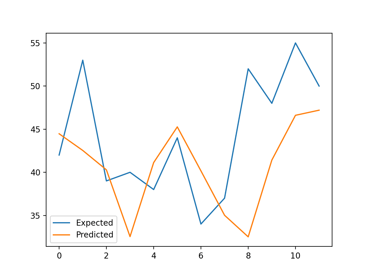
Line Plot of Expected vs. Births Predicted Using XGBoost
Once a final XGBoost model configuration is chosen, a model can be finalized and used to make a prediction on new data.
This is called an out-of-sample forecast, e.g. predicting beyond the training dataset. This is identical to making a prediction during the evaluation of the model: as we always want to evaluate a model using the same procedure that we expect to use when the model is used to make prediction on new data.
The example below demonstrates fitting a final XGBoost model on all available data and making a one-step prediction beyond the end of the dataset.
# finalize model and make a prediction for monthly births with xgboost
from numpy import asarray
from pandas import read_csv
from pandas import DataFrame
from pandas import concat
from xgboost import XGBRegressor

# transform a time series dataset into a supervised learning dataset
def series_to_supervised(data, n_in=1, n_out=1, dropnan=True):
	n_vars = 1 if type(data) is list else data.shape[1]
	df = DataFrame(data)
	cols = list()
	# input sequence (t-n, ... t-1)
	for i in range(n_in, 0, -1):
		cols.append(df.shift(i))
	# forecast sequence (t, t+1, ... t+n)
	for i in range(0, n_out):
		cols.append(df.shift(-i))
	# put it all together
	agg = concat(cols, axis=1)
	# drop rows with NaN values
	if dropnan:
		agg.dropna(inplace=True)
	return agg.values

# load the dataset
series = read_csv('daily-total-female-births.csv', header=0, index_col=0)
values = series.values
# transform the time series data into supervised learning
train = series_to_supervised(values, n_in=6)
# split into input and output columns
trainX, trainy = train[:, :-1], train[:, -1]
# fit model
model = XGBRegressor(objective='reg:squarederror', n_estimators=1000)
model.fit(trainX, trainy)
# construct an input for a new preduction
row = values[-6:].flatten()
# make a one-step prediction
yhat = model.predict(asarray([row]))
print('Input: %s, Predicted: %.3f' % (row, yhat[0]))
Running the example fits an XGBoost model on all available data.
A new row of input is prepared using the last 6 months of known data and the next month beyond the end of the dataset is predicted.
Input: [34 37 52 48 55 50], Predicted: 42.708
Further Reading
This section provides more resources on the topic if you are looking to go deeper.
Related Tutorials
- A Gentle Introduction to the Gradient Boosting Algorithm for Machine Learning
- Time Series Forecasting as Supervised Learning
- How to Convert a Time Series to a Supervised Learning Problem in Python
- How To Backtest Machine Learning Models for Time Series Forecasting
Summary
In this tutorial, you discovered how to develop an XGBoost model for time series forecasting.
Specifically, you learned:
- XGBoost is an implementation of the gradient boosting ensemble algorithm for classification and regression.
- Time series datasets can be transformed into supervised learning using a sliding-window representation.
- How to fit, evaluate, and make predictions with an XGBoost model for time series forecasting.
Do you have any questions?
Ask your questions in the comments below and I will do my best to answer.
The post How to Use XGBoost for Time Series Forecasting appeared first on Machine Learning Mastery.